[논문 Summary] SNGAN (2018 ICLR) "Spectral Normalization for Generative Adversarial Networks"

[논문 Summary] SNGAN (2018 ICLR) "Spectral Normalization for Generative Adversarial Networks"

 

목차

 

논문 정보

Citations : 2022.02.23 기준 2822 회

저자

Takeru Miyato, Toshiki Kataoka - Preferred Networks, Inc. 
Masanori Koyama - Ritsumeikan University 
Yuichi Yoshida - National Institute of Informatics

논문 링크

ICLR 2018 Conference 원본 논문

https://openreview.net/forum?id=B1QRgziT- 

Spectral Normalization for Generative Adversarial Networks

 

Ian Goodfellow의 Twitter

 

논문 Summary

 

Abstract

 

GAN 학습에 있어 훈련의 불안정성이 문제로 대두되고 있음.

이에 discriminator의 훈련을 안정화시킬 수 있는 spectral normalization을 새롭게 제안함.

이를 통해 계산량이 줄어들고 쉽게 적용할 수 있으며 학습의 안정성을 꾀함.

이에 대한 실험적으로 그 증명을 대신함.

 

1. Introduction

 

1문단 : (GAN의 특징과 소개)

 

GAN의 훈련에 있어 지속적인 어려움은 discriminator의 성능 제어에 달려있다. 모델 분포와 target 분포가 불일치 혹은 겹치는 곳이 없어 discriminator가 빠르고 잘 구분되는 순간에 도달하면 generator의 훈련도 멈추기 때문에 문제가 된다. 

 

본 논문에서 discriminator 네트워크의 훈련을 안정화시킬 수 있는 spectral normalization이라 불리는 새로운 weight normalization 방법을 제안한다. 2가지 속성은 다음과 같다.

1) Lipschitz constant는 조절해야할 유일한 hyper-parameter이다. 이 마저도 별도의 tuning이 필요없음.

2) 간단하게 적용할 수 있고 추가적인 계산 비용은 작다.

 

이 논문에서는 weight normalization , weight clipping(WGAN), gradient penalty(WGAN-GP)와 같은 다른 regularization 기법들과 비교할 예정이고 정성적으로 효용성이 높음을 증명할 예정이다.

 

2. Method

 

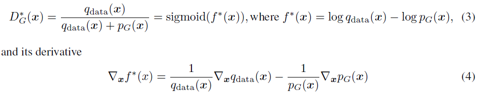
GAN에 있어 최적의 Discriminator는 위와 같이 표현할 수 있으며 그 미분은 Eq (4)와 같다.

$sigmoid(x)={1 \over 1 + e^{-x}}$이기 때문에 $f^*$을 sigmoid에 넣어 풀면 $D_G^*$와 같이 가능하다. 그러나 해당 방법론은 boundary를 고려하지 않는다. (즉, 다시 말하면 Lipschitz continuity를 고려하지 않는다.)

 

최근 machine learning 집단에서의 GAN의 성능은 Lipschitz continuity를 통한 boundary를 고려한 통계를 기반으로 훈련을 진행한다. 특히, regularization term을 추가함으로써 discriminator의 Lipschitz constant 를 제어하기 위해 많은 방법들이 제안되었다. 

$ {\lVert f(x) - f(x^\prime) \rVert \over \lVert x - x^\prime \rVert}  \le M$ 여기서 M은 작은 값 보통은 1이고 norm은 $l_2$ norm

https://lernapparat.de/more-improved-wgan/

 sample 기반의 수식은 상대적으로 간단하게 regularization이 가능하지만 heuristic 방법 없이 데이터 분포와 생성기의 지원 공간 밖에 있는 곳에 대한 regularization을 내제하게 하는 것은 어렵다. (즉, 함수 공간 전체에 대한 regularization이 어렵다) 이에 spectral normalization이라는 weight matrix normalizing을 통해 이런 문제를 회피하고자 한다.

 

2.1 Spectral Normalization

 

Spectral normalization은 각 layer $g$의 spectral norm을 제어함으로써 discriminator 함수 $f$의 Lipschitz constant를 제어하는 것이다.

Lipschitz norm $\lVert g \rVert_{Lip}= sup_h \sigma (\nabla g(h))$. 여기서 $\sigma (A)$ 중 A는 spectral norm을 적용한 행렬이고 $L_2$ 행렬의 norm

식 (6)은 A의 가장 큰 singular value와 동치

linear layer $g(h)=Wh$라 함은 $\lVert g \rVert_{Lip}= sup_h \sigma (\nabla g(h)) = sup_h \sigma (W)= \sigma(W)$이고 activation fuction의 Lipschitz norm은 1로 설정. Inequality인 $\lVert g_1 \circ g_2 \rVert_{Lip} \le \lVert g_1 \rVert_{Lip} \cdot \lVert g_2 \rVert_{Lip}$에 의거하여 다음과 같은 수식이 나옴.

 

 

Spectral Noramzliation은 Weight matrix $W$의 Spectral norm을 정규화하여 $\sigma(W)=1$을 만족한다.

 

 식 (7)과 식 (8)에 의거하여 $\lVert f \rVert_{Lip}$가 1로 bound됨. 

 

2.2 Fast Approximation of the Spectral Norm $\sigma(W)$

$\sigma(W)$에 대한 계산을 위해 순진하게 singular value decomposition(SVD)를 진행할 시 계산량이 매우 많다. 따라서 power iteration method를 통해 $\sigma(W)$ 추정하는 것이 더 효율적이다. 이와 관련해서는 Appendix A- Algorithm 1을 참조

 

2.3 Gradient Analysis of the Spectrally Normalized Weights

 

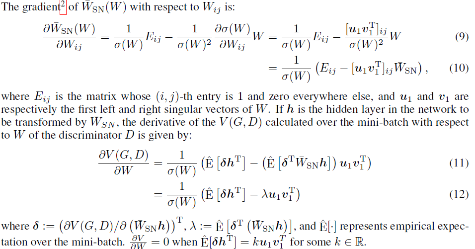
 Spectral Normalization을 적용시킨 Weight matrix에 대한 미분을 진행하면 식 (9)와 (10)과 같이 나타낼 수 있다. 이를 V를 기반으로 미분하면 식 (11)과 (12)와 같다. mini-batch로 학습할 경우 다 합쳐서 loss를 업데이터 하기 때문에 Expectation을 사용한다.

갑작스럽게 수식이 점프된 것이 헷갈릴 수 있어 추가적인 식을 쓰면 다음과 같다

$${\partial V(G,D) \over \partial W_{i,j}} = {\partial V(G,D) \over \partial \bar{W}_{SN} h }{\partial \bar{W}_{SN} h \over \partial W_{i,j}} = \delta {\partial \bar{W}_{SN} \over \partial W_{i,j} }h$$

이 식에서 식 (10)을 대입하면 식 (12)를 도출할 수 있다.

 

식 (12)에서 해석을 표현해보면 다음과 같다.

첫 번째 term $\hat{E} [\delta h^T]$는 normalization이 없는 weight 미분과 같다.

두 번째 term은 adaptive regularization coefficient인 $\lambda$와 첫 번째 singular component를 penalize하는 term이다. 이때 $\lambda$가 양수는 $\delta$와 $\bar{W_{SN}}h$가 비슷한 방향을 가르키고 있다는 말이고 이를 다시 풀이하면 W의 column spacec가 한 방향으로 집중되어 훈련되는 것을 막아준다.

정리하면 Spectral normalization이 각 layer의 변형이 한 방향으로 민감하게 되는 것을 방지한다. 즉, 다양한 방향으로 다양한 함수 공간으로의 관점을 보기를 원하는 것이다.

 

3. Spectral Normalization Vs Other Regularization Techniques

 

Weight Normalization (2016 NIPS)

 

2016년 Salimans & Kingma가 NIPS에서 제안한 weight normalization은 weight matrix에서 각 행 벡터를 $l_2$ norm으로 정규화하는 것이다.

 

weight normalization은 의도와 달리 행렬에 너무 강한 제약을 줘서 rank가 1이 되게한다. (첫 번째 singular value만 존재하고 나머지는 0) 즉, target으로부터 모델 확률 분포를 오직 하나의 feature만을 가지고 판별한다. weight clipping 역시 비슷한 문제를 가지고 있으나 Spectral normalization은 rank에 독립적이기 때문에 1-Lipschitz constrain을 만족하면서 matrix에 많은 feature들을 사용할 수 있게 한다.

 

Orthonormal regularization (2016) 

각 weight별로 orthonormal regularization을 도입함으로써 GAN 훈련을 안정시킬 수 있다. 그러나 모든 singular value를 1로 제약하기 때문에 spectrum에 대한 정보를 파괴하는 문제가 생긴다. spectrul normalization은 spectrum의 scale만 조율해 최대값을 1로 설정하기 때문에 다르다. 

 

Gradient Penalty (2017 NIPS WGAN-GP)

 

위에서 언급한 문제점들은 없지만 생성 분포의 support에 의존적이라는 것이 문제이다. 왜냐하면 해당 분포는 계속 바뀌기 때문. 그리고 경험적으로 높은 learning rate는 WGAN-GP의 성능을 분안정하게 한다. spectral normalization은 안정적. 또한, WGAN-GP는 spectral normalization과 달리 한 번에 forward & backward 를 처리해야하기 때문에 계산량이 많다.

 

4. Experiments

CIFAR 10과 STL 10, ImageNet을 통한 결과를 보인다.

(objective function에 대한 설명 생략)

inception score & FID를 통한 정량적 평가 진행

4.1 Results on CIFAR 10 and STL-10

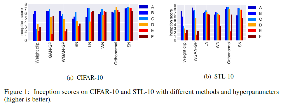
6개의 hyper-parameter에 대한 값들을 변형시시켜 각 모델별로 비교를 진행함.

$\alpha$는 learning rate, $\beta_1, \beta_2$는 Adam optimizer의 momentum parameter 1, 2차 계수, $n_{dis}$는 한 번 generator update마다 시행할 discriminator update 횟수를 의미.

 

각 모델은 Weight Clipping(WGAN), GAN-GP, WGAN-GP, BN(Batch Normalization), LN(Layer Normalization), WN(Weight Normalization), Orthonormal Regularization 그리고 마지막으로 SN(Spectral Normalization)

 

모든 실험은 100K iteration

 

Table 1에서 설명하는 양 데이터 세트 모든 hyper-paramter에 대해 다른 모델들 대비 강건한 점수를 Figure 1에서 보여줌.

 

Figure 2 역시 마찬가지로 SN이 좋은 성과를 보여줌.

 

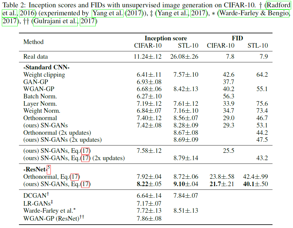
정량적으로 봤을 때 언제나 완벽하게 최상의 결과를 나타낸다고 보장하기에는 어려우나 대다수의 경우 최상의 결과를 도출함을 확인할 수 있다.

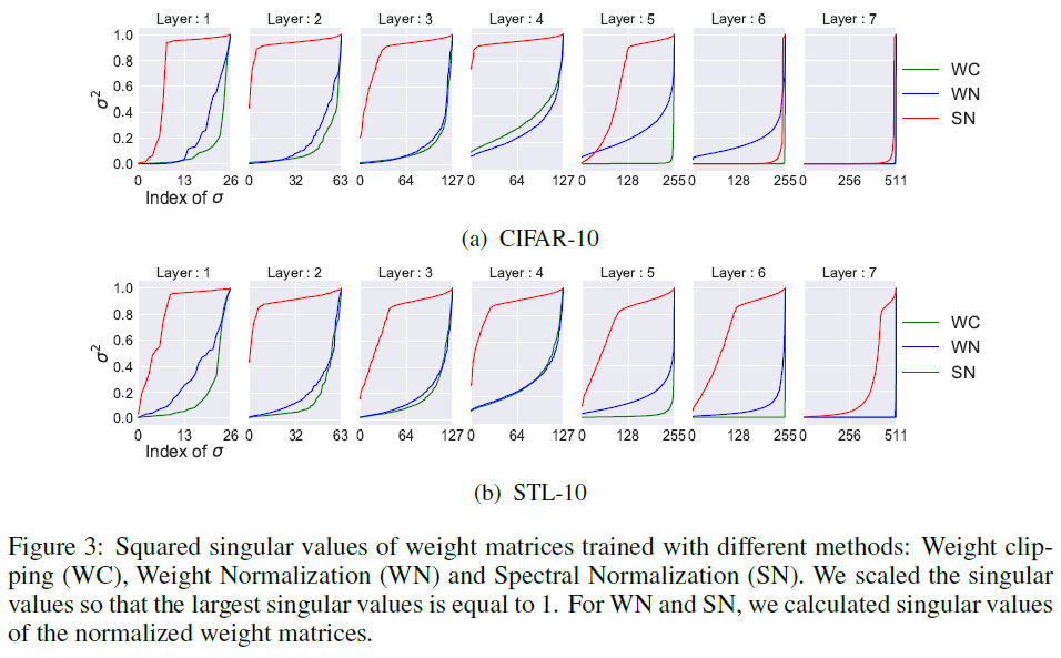
Figure 3는 모든 layer에 대한 Spectral Normalization이 빠르게 1에 가깝게 도달한 singular value들을 계산함으로 보여준다.

Training Time : Spectral Normalization은 weight normalization보다 약간 느리지만 WGAN-GP보다는 상당히 빠르다. 

 

 Section 3에서 언급한 바와 같이 Orthonormal regularization은 모든 feature 차원을 1로써 동등하게 강조함으로써 spectral information을 파괴한다. 때문에 Figure 4에서 나타난 것과 마찬가지로 feature map dimiension size가 커지면 orthonormal의 성능은 악화되는 반면 SN-GAN은 균일한 성능을 보임을 확인한다.

 

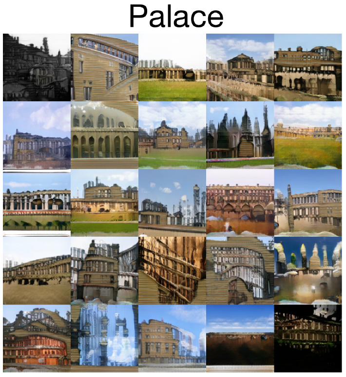
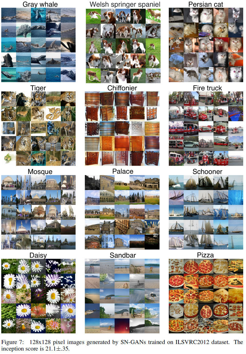
4.2 Image Generation on ImageNet

 

1300 이미지로 구성되고 1000개의 클래스를 가지는 ImageNet에서 cGAN의 훈련에 있어 128x128 사이즈로 압축하여 사용한다.

Appendix B.3에 설정이 나와있다.

 

 

 

5. Conclusion

GAN읜 훈련을 안정화시킬 수 있는 spectral normalization을 제안한다. 생성된 이미지는 weight normalization을 적용한 것보다 다양한 이미지를 생성하고 상대적으로 높거나 견줄만한 inception score를 획득한다. discriminaotr에 전역적인 regularization을 내제한다.

 

Reference

 

공식 Github

https://github.com/pfnet-research/sngan_projection

GitHub - pfnet-research/sngan_projection: GANs with spectral normalization and projection discriminator

 

 

도움이 되는 YouTube 

https://youtu.be/iXSYqohGQhM

 

이를 정리한 블로그 

https://aigong.tistory.com/370

PR-087 "Spectral Normalization for Generative Adversarial Networks" Review (2018 ICLR)(GAN)

 

https://jaejunyoo.blogspot.com/2018/05/paper-skim-spectral-normalization-for-gan.html

[Paper Skim] Spectral Normalization for Generative Adversarial Networks

https://jonathan-hui.medium.com/gan-spectral-normalization-893b6a4e8f53

GAN — Spectral Normalization