[논문 Summary] Neural Style Transfer (2016 CVPR) "Image Style Transfer Using Convolutional Neural Networks"

[논문 Summary] Neural Style Transfer (2016 CVPR) "Image Style Transfer Using Convolutional Neural Networks"

 

목차

 

 

논문 정보

 

Citation : 2022.02.10 목요일 기준 3527회

 

저자 

 

Leon A. Gatys / Alexander S. Ecker / Matthias Bethge

- Centre for Integrative Neuroscience, University of T¨ubingen, Germany / Bernstein Center for Computational Neuroscience, T¨ubingen, Germany

 

 

논문 Summary

 

논문 리뷰는 각 section별로 요약할 것이고 중간중간 저의 생각과 아이디어가 추가되는 식으로 진행할 것입니다.

(직접 짠 코드 리뷰는 추후 링크를 통해 확인하시길 바랍니다.)

본 논문은 이미 학습된(pretrained) VGG network의 feature map들을 활용하여 content image와 style image의 정보를 input image에 줌으로써 학습을 진행하는 Texture Transfer (혹은 Style Transfer) 알고리즘 소개하는 초창기 논문입니다. 이때 사용하는 다양한 방법에 대해 간략하게 보도록 하겠습니다.

 

1. Introduction

 

본 위치에서는 일반 논문으로 치면 Introduction과 Related Work를 섞은 파트로 전반적인 style transfer에 대한 이야기를 하고 있습니다.

 

우선 논문 서두부터 한 이미지의 style을 다른 image로 전달하는 것을 texture transfer 문제라고 정의한다. 초창기 texture transfer는 non-parametric algorithm을 통해 texutre 합성을 진행할 수 있었지만 여기에는 low-level feature만을 사용한다는 한계점이 존재한다. 

 

이상적인 style transfer algorithm은 target image로부터 중요한 이미지 content를 뽑아내고 source image의 스타일을 정제하여 texutre transfer procedure에 전달할 수 있어야 한다. 

 

일반적으로 원본 이미지의 style로부터 content를 분리시키는 일은 매우 어려운 문제이지만 Deep Convolutional Neural Network는 이미지의 high-level semantic information을 추출할 수 있기 때문에 style transfer가 가능하다.

 

본 연구에서 style transfer를 수행할 수 있는 새로운 알고리즘 "A Neural Algorithm of Artistic Style"에 대해 소개하고자 한다. CNN을 통해 style과 content를 독립적으로 처리하고 조작함으로써 이를 가능하게 한다.

 

2. Deep image representations

 

본 위치에서는 보통 모델의 구성 방법과 소개에 대해 말하고 있습니다.

 

본 결과는 VGG network를 기반으로 생성되어진다.

 

저자들은 16개의 CNN과 5개의 Pooling layer로 구성된 VGG19에서 normalized된 version의 feature map을 활용한다. (이 부분은 코드 실습에 중요하니 기억)

 

또한, fully conneted layer는 사용하지 않으며 caffee-framework로 짠 코드가 공개되어 있다. (저자들의 코드는 Reference 1-2)를 참조. 그러나 lua로 되어있어 볼 사람들만 보는 것을 추천함.)

 

이미지 합성을 위해 max pooling 대신 avg pooling이 더 나은 결과를 도출한다는 것을 발견했다. (이 부분은 선택사항입니다. 필요한 분은 추후 코드에서 avg pooling으로 바꾸시면 됩니다. 이 부분은 parameter가 없으므로 바꿔도 무방합니다.)

 

Pytorch 코드적으로는 아래의 코드를 maxpooling 대신 교체할 수 있다.

avgpool = nn.AvgPool2d(kernel_size=layer.kernel_size, 
                       stride=layer.stride, 
                       padding=layer.padding)

  

2.1 Content representatio

 

Notation에 대해 먼저 설명하면 다음과 같다.

 

$N_l$ : 한 layer의 filter 수로 channel의 수 

$M_l$ : feature map의 높이(Height)와 너비(Width)의 곱

$F_{i,j}^l$ : layer l에서 j번째 위치에 존재하는 i번째 filter의 activation으로 생각할 수 있고 $F^l \in R^{N_l \times M_l}$으로 표기 가능하다.

$\vec{p}$ : content original image 원본 이미지

$\vec{x}$ : 생성된 image 

$P^l$ : content original image에서 layer l에 위치하는 feature map

$F^l$ : 생성된 이미지에서 layer l에 위치하는 feature map

 

이때 우리는 content image에 대한 학습을 위해 원본 이미지와 생성된 이미지 간 MSE Loss를 활용한다. 그것이 바로 아래 식 (1)이다.

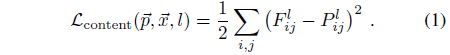
식 (1)을 미분하면 다음과 같이 나타낼 수 있다. 

 

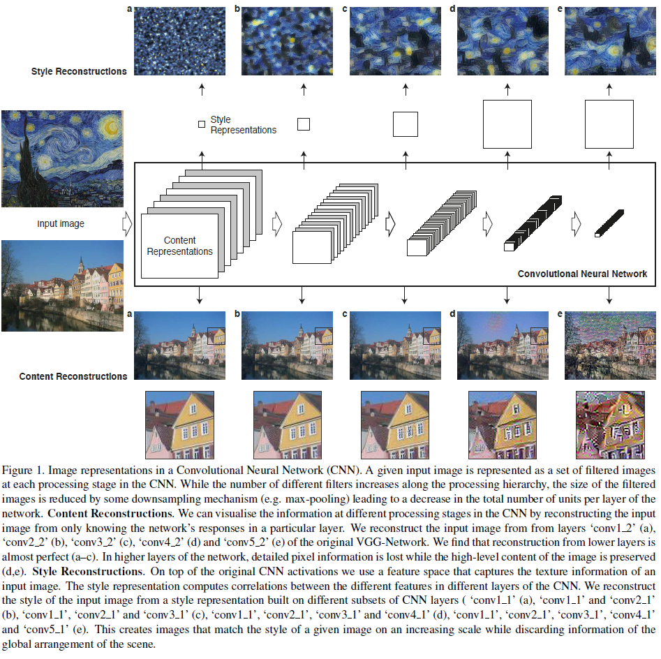
다만 이때 network의 higher layer (Figure 1. d와 e)는 물체나 정렬에 대한 high-level content를 포착하고 lower layer(Figure 1. a-c)는 단순히 원본 이미지의 정확한 픽셀 값을 재생산하는데 초점이 맞춰져 있다. 여기서 저자들은 higher layer의 feature map을 content representation을 위한 방식으로 활용한다.

cf) 코드 상에서는 d정도 위치에 존재하는 3번째 pooling layer 이후의 4_2 conv layer를 content layer의 feature map으로 활용한다. 해당 내용은 뒤 Figure 2와 2.2에서 설명한다.

 

2.2 Style representation

 

input image의 style 표현을 획득하기 위해서는 feature space에서의 정보를 활용할 필요가 있다. 이때 활용하는 것이 바로 Gramm matrix $G^l$이다. 

$$G^l \in R^{N_l \times N_l}$$

$G_{i,j}^l$은 layer l에서 vector화된 feature map i와 j간 내적을 한 것으로 식 (3)과 같이 표기한다.

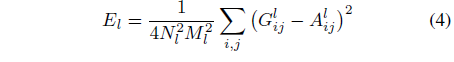
저자들은 원본이미지의 Gram matrices와 생성된 이미지의 Gram matrices 간 mean-squared distance를 최소화하는 방향으로 Loss를 구성한다. (코드에서 style loss 짤 때 중요)

 

Gram matrix

만약 Gram matrix에 대해 자세히 들여다보고 싶다면 아래 링크 참조

https://aigong.tistory.com/360

Gram matrix (그람 행렬) 정리

 

앞에서는 content original image로 $\vec{p}$를 사용했다면 여기서 style을 학습하기 위한 style original image로 $\vec{a}$를 사용한다. 당연히 layer l에 대한 feature representation 역시 $A^l$로 표기한다.

 

$\vec{a}$ : style original image

$\vec{x}$ : 생성된 image 

$A^l$ : style original image에서 layer l에 위치하는 feature map

$F^l$ : 생성된 이미지에서 layer l에 위치하는 feature map

 

 Total style loss는 다음과 같이 표기한다.

 

이때, $w_l$ 은 style loss를 위한 각 layer별 weighting factor이다. (코드에서 중요. 추후 설명이 나오겠지만 0.2를 잡음.) 

 

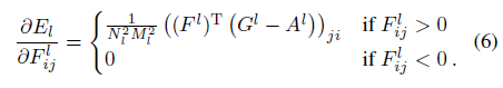
식 (5)를 미분하면 다음과 같은 식을 도출할 수 있다.

 

 

 

2.3 Style Transfer

 

정리하면 우리는 input image $\vec{x}$에 content 정보를 가진 $\vec{p}$와 style 정보를 가진 $\vec{a}$를 합성하고 싶은 것이다. 이를 위한 최종적인 loss function은 식 (7)과 같다.

 

 

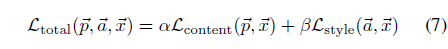
이때, $\alpha , \beta$는 content와 style reconstruction의 weighting factor를 각각 나타낸 것이다.

optimizer로 L-BFGS를 사용한다. 

 

cf) 코드상으로는 Adam도 가능하나 개인적으로 구성한 코드에서는 L-BFGS를 사용했다. 이때 코드 상의 차이점이 약간 존재하므로 유의

 

그리고 저자들은 style image와 content image의 사이즈는 같게 항상 resize한다.

 

3. Results

본 위치에서는 각종 실험에 대한 결과를 기술한다.

 

Style Transfer 알고리즘을 도식화한 Figure는 Figure 2이다.

 

 보이는 바와 같이 content image와 style image가 존재하고 우리가 생성할 이미지 $\vec{x}$는 white noise부터 시작해서 content의 정보와 style 정보를 합성하여 얻어낸다. 모두 동일하게 pretrained VGG network를 활용하며 이때의 학습은 VGG network이 아니라 input image $\vec{x}$가 backprop되면서 점차 변화하는 것을 의미한다.

 

 

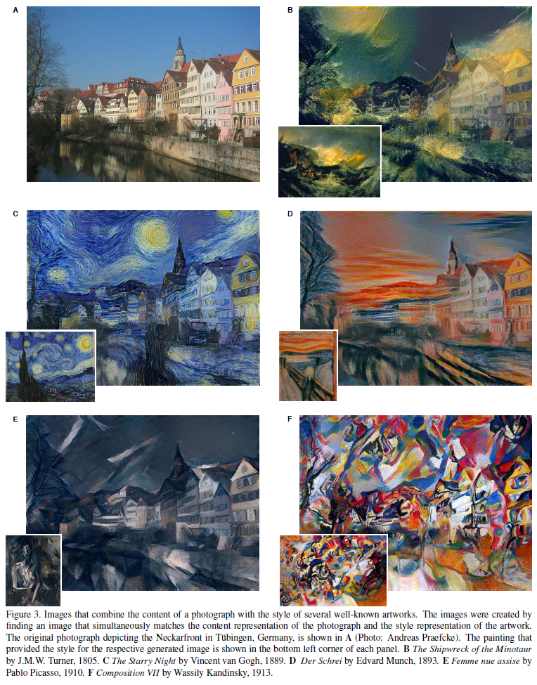
Figure 3를 위해서 어떤 layer를 사용할지 정해야 하는데 본 논문에서는 다음과 같이 정해서 사용했다고 한다.

1) content representation을 위해서 단일 layer 즉, 'conv4_2' layer만을 사용

2) style representation을 위해서 5개의 layer 즉, 'conv1_1', 'conv2_1', 'conv3_1', 'conv4_1', 'conv5_1' layer들을 사용

 

VGG network layer별 conv naming

 

 

 

 

 

이때,

식 5에서 설명한 style loss weighting factor $w_l$은 위 layer에 대해 0.2를 설정했다.

식 7에서 설명한 content와 style reconstruction의 weighting factor인 $\alpha , \beta$에 대해 비율을 설정하는데 이때 Figure 3에 대한 그림별로 상이하다.

$\frac{\alpha}{\beta}$의 비율

Fig 3. B $\frac{\alpha}{\beta} = 1 \times 10^{-3}$

Fig 3. C $\frac{\alpha}{\beta} = 8 \times 10^{-4}$

Fig 3. D $\frac{\alpha}{\beta} = 5 \times 10^{-3}$

Fig 3. E, F $\frac{\alpha}{\beta} = 5 \times 10^{-4}$

 

논문에서는 비율만 나와있고 따로 값에 대한 설명이 없어 코드에서 $\alpha$는 1로 놓고 나머지는 $\beta$로 설정했다. 고로 Fig 3. B에서 $\frac{\alpha}{\beta} = 1 \times 10^{-3}$이므로 $\alpha = 1, \beta=10^3$으로 setting함.

 

다만 실험에서는 상황에 따라 값을 올리는 경우가 좋았던 경우가 있음. 이는 3.1과 관련 있음

 

3.1 Trasde-off between content and style matching

 

Figure 4.에서 보이는 바와 같이 content와 style image의 weighting factor의 비율 즉, $\frac{\alpha}{\beta}$의 비율을 변화시켰을 때의 변화 정도를 확인할 수 있다. 만약 그 값의 정도가 강해진다. 즉, 오른쪽 아래처럼 $10^{-1}$이 된다면 content의 정보가 더 강해지는 것을 확인할 수 있고 만약 그 값의 정도가 약해진다. 즉, 왼쪽 위처럼 $10^{-4}$이 된다면 style 정보가 강해지는 것을 확인할 수 있다.

 

style 정보를 강하게 넣고싶다면 $\beta$의 값을 높히거나 $\alpha$의 값을 낮히면 된다.

content 정보를 강하게 넣고싶다면 $\beta$의 값을 낮히거나 $\alpha$의 값을 높히면 된다.

 

그러나 실험에서는 $\alpha = 1$로 고정시키므로 $\beta$의 값으로 조절한다.

 

이 trade-off관계를 여기서는 제목과 같이 표현한 것

 

3.2 Effect of different layers of the Convolutional Neural Network

 

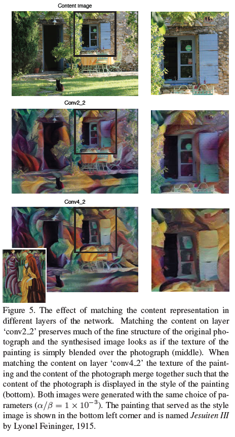
Figure 5에서 나와있듯, conv 2_2와 같은 lower layer는 더 구체적인 pixel 정보를 함유하고 있어 원본 이미지의 구조를 답습하지만 conv4_2와 같은 higher layer는 구조에 대한 큰 제약 없이 style과 잘 섞이도록 함을 보이고 있다.

즉, style transfer를 위해서는 higher layer를 활용하는 편이 style과 잘 섞이는 방법 중 하나이다.

 

3.3 Initialization of gradient descent

 

 

Figure 6 C에서 보이듯, 본 논문에서 초기 input image는 white noise로 시작한다. 

그러나 Figure 6. A처럼 content image로부터 시작할 수도 있고 Figure 6. B처럼 style image로부터 시작할 수도 있다.

 

다만, white noise image로 시작한 이미지는 모두 다양한 새로운 이미지를 생성한 것에 반해 content image나 style image로 초기화해서 진행한 style transfer image는 모두 같은 결과를 가진다.

 

즉, 다양한 새로운 이미지를 보고싶다면 white noise로 시작하는 방법을 할 것을 권장함

3.4 Photorealistic style transfer

 

시차를 바꾸는 이미지 합성으로 style transfer를 활용할 수 있다.

 

4. Discussion

 

본 알고리즘은 분명 높은 지각적 질적 결과를 보여주지만 기술적 결함이 존재한다.

1) Resolution

특히, 해상도와 관련한 부분이 문제로 본 논문에서는 512x512의 이미지 해상도를 가지고 NVIDIA K40 GPU로 한시간을 투자하여 결과를 얻어낸다. 즉, 이미지의 해상도가 합성 결과를 나타내는 속도를 결정짓는다.

 

2) low-level noise

 

 

대다수의 작업이 확실히 style과 content image를 완벽하게 분리했는지 또 그것을 설명할 수 있는지가 분명하지 않다. 그럼에도 불구하고 우리는 Neural system을 활용한 style transfer를 제안하고 있기에 이를 더 잘 설명할 수 있는 확장이 필요하다.

 

 

 

 

직접 구현한 코드의 결과

 

 

 

 

Other Reference

 

1-1) Leon A. Gatys의 공식 Github : Lua 파일로 된 style transfer

 

https://github.com/leongatys/fast-neural-style

GitHub - leongatys/fast-neural-style

 

1-2) Leon A. Gatys의 공식 Github : Pytorch 파일로 된 style transfer

 

https://github.com/leongatys/PytorchNeuralStyleTransfer

GitHub - leongatys/PytorchNeuralStyleTransfer: Implementation of Neural Style Transfer in Pytorch

 

2-1) Pytorch Tutorial (영문)

https://pytorch.org/tutorials/advanced/neural_style_tutorial.html?highlight=neural 

Neural Transfer Using PyTorch — PyTorch Tutorials 1.10.1+cu102 documentation

 

2-2) Pytorch Tutorial (국문)

https://tutorials.pytorch.kr/advanced/neural_style_tutorial.html?highlight=neural%20transfer 

PyTorch를 이용하여 뉴럴 변환(Neural Transfer) — PyTorch Tutorials 1.10.2+cu102 documentation

 

3. Tensorflow Tutorial 

https://www.tensorflow.org/tutorials/generative/style_transfer

tf.keras를 사용한 Neural Style Transfer  |  TensorFlow Core

 

4. 블로그

https://towardsdatascience.com/implementing-neural-style-transfer-using-pytorch-fd8d43fb7bfa

Implementing Neural Style Transfer Using PyTorch